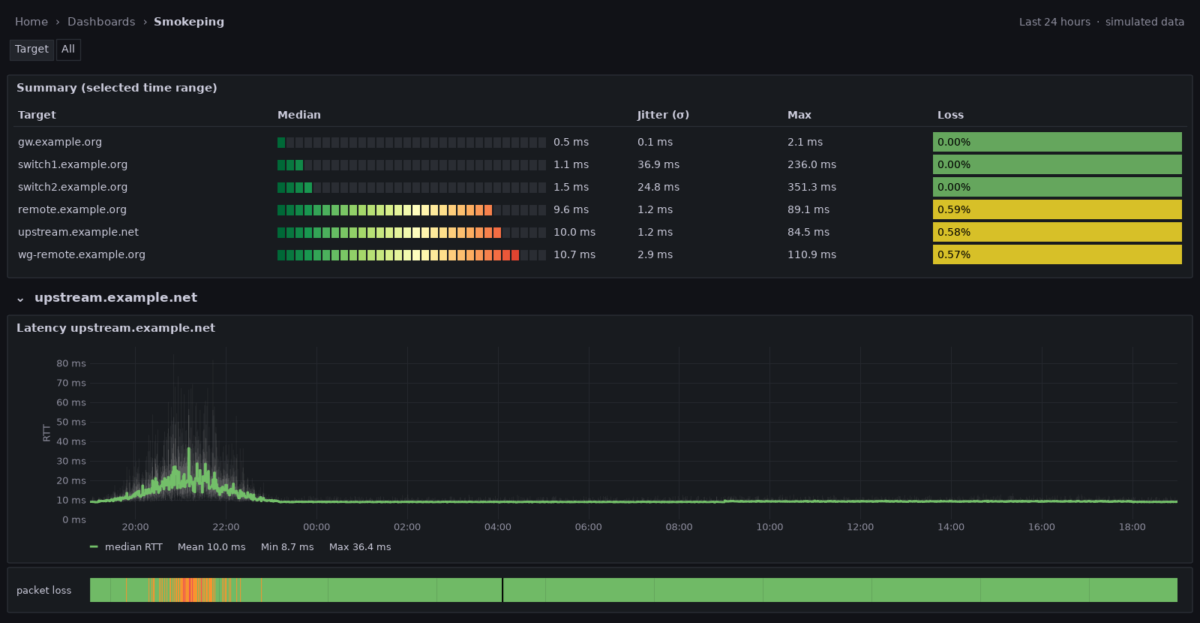
SmokePing without SmokePing: latency smoke graphs with Telegraf, InfluxDB and Grafana – Linux

Few monitoring graphs are as instantly readable as SmokePing‘s: a green line for the median round-trip time, grey “smoke” around it showing how far the individual pings scattered, and colour for packet loss. A thin line means a calm link. A tall, light cloud means jitter, even when the average looks fine.

My monitoring stack already runs Telegraf, InfluxDB and Grafana, and I didn’t want another daemon with its own RRD files and web frontend next to it. So I rebuilt the SmokePing view from what was already there: Telegraf’s ping input as the probe, InfluxDB for storage, and a Grafana dashboard that draws the smoke. This post covers the probe, the dashboard, and two traps that silently cost me half of my samples.

Grafana Smokeping dashboard over 24 hours with simulated data: a summary table of six targets, then the latency graph of upstream.example.net. The median sits at about 9 ms all day except in the evening, when it rises to 20 to 36 ms around 21:00 with tall grey smoke up to 80 ms; the packet-loss strip below turns yellow, orange and red during that time and shows a short black mark at 04:05. — The dashboard over 24 hours (simulated data, see below): evening congestion on the upstream path and a short nightly reconnect at 04:05.

What SmokePing actually measures

The trick behind the smoke is simple. SmokePing doesn’t send one ping now and then. It sends a burst of 20 pings per target (every 5 minutes by default), sorts the 20 round-trip times, and plots their distribution: the median as a line, the rest as shades of grey. Where many pings landed the smoke is dark, where only a few outliers went it is light. Lost pings colour the median line.

So to rebuild it I need two things: a probe that sends bursts and keeps the distribution, not just an average, and a graph that can fill the space between two series.

The probe: Telegraf’s ping input

Telegraf’s inputs.ping can do both. With method = "native" it uses its own ICMP implementation instead of calling the system ping binary, and only in that mode it can also calculate percentiles of each burst. That’s exactly the distribution the smoke needs.

# /etc/telegraf/telegraf.d/smokeping.conf
[[inputs.ping]]
  ## one burst per minute (SmokePing: every 5 minutes)
  interval = "60s"

  urls = [
    "gw.example.org",                   # firewall / LAN gateway
    "switch1.example.org",              # LAN switches
    "upstream.example.net",             # upstream reference
    "remote.example.org",               # remote server, direct
    "wg-remote.example.org",            # same server through WireGuard
  ]

  method = "native"

  ## 20 pings, one second apart
  count = 20
  ping_interval = 1.0

  ## total runtime of one burst, see below
  deadline = 25

  ## distribution of the 20 round-trip times
  percentiles = [10, 25, 50, 75, 90]

  [inputs.ping.tags]
    probe = "smokeping"

Each burst becomes one point in the ping measurement, tagged with the target in url. The fields that matter for the dashboard are minimum_response_ms, percentile10_ms to percentile90_ms, maximum_response_ms, standard_deviation_ms, packets_transmitted and percent_packet_loss. One burst per minute is denser than SmokePing’s default, which makes short incidents visible. Grafana aggregates the points again for longer time ranges anyway.

Trap 1: raw sockets

On the first start, Telegraf only logged this, once per target and minute:

E! [inputs.ping] ping failed: permission changes required, enable CAP_NET_RAW
capabilities or use unprivileged ping (refer to the ping plugin's README.md for more info)

The native mode opens raw ICMP sockets, and the package’s systemd unit runs Telegraf as the unprivileged user telegraf. The fix that survives package updates is a systemd drop-in. setcap on /usr/bin/telegraf also works, but every package update replaces the binary and silently drops the capability again.

linux # sudo systemctl edit telegraf

[Service]
AmbientCapabilities=CAP_NET_RAW

sudo systemctl daemon-reload && sudo systemctl restart telegraf

If your unit already sets CapabilityBoundingSet for other plugins, add CAP_NET_RAW to it rather than replacing it. When Telegraf runs in Docker, cap_add: [NET_RAW] does the same job.

Trap 2: timeout is not deadline

My first config had timeout = 1.0, copied from the exec-mode examples. Telegraf accepted it with only a warning:

W! [inputs.ping] "timeout" is ignored when method = "native"; use "deadline" to control the total runtime

Easy to dismiss, but the data told a different story. In native mode, deadline limits the whole burst, and its default is 10 seconds. 20 pings one second apart need about 20. Every burst was cut off halfway: packets_transmitted was 10, not 20. Worse, now and then an 11th ping left just before the cut-off and its reply never got counted, so a perfectly healthy target showed 1 lost packet out of 11, which is 9.1 % fake packet loss. With deadline = 25 (20 pings plus some time for the last reply) every burst now reports 20 sent and 20 received.

The lesson: after setting up a probe, check packets_transmitted, not just whether data arrives.

Drawing the smoke in Grafana

Grafana’s time series panel has no “smoke” mode, but it has Fill below to: a series can fill the area down to another series instead of down to zero. Three pairs of series, each filled to its partner in grey with increasing opacity, give the layered smoke:

Band	Upper series	Fill below to	Fill opacity
all 20 pings	max	min	12 %
middle 80 %	p90	p10	22 %
middle 50 %	p75	p25	40 %

All six band series get line width 0 and are hidden from the legend. The median is the only visible line: green, 2 px. With step after interpolation each burst shows as a flat block, which matches what a burst is: one measurement for one minute.

The queries are plain Flux. Min and max are aggregated with min and max so a zoomed-out view doesn’t average the outliers away. The percentiles use mean and get short names that the overrides match on:

import "strings"

from(bucket: "telegraf")
  |> range(start: v.timeRangeStart, stop: v.timeRangeStop)
  |> filter(fn: (r) => r._measurement == "ping" and r.url == "${target}"
                       and r._field =~ /^percentile(10|25|50|75|90)_ms$/)
  |> aggregateWindow(every: v.windowPeriod, fn: mean, createEmpty: false)
  |> map(fn: (r) => ({_time: r._time, _value: r._value,
        _field: if r._field == "percentile50_ms" then "median"
                else "p" + strings.replaceAll(v: strings.replaceAll(v: r._field, t: "percentile", u: ""), t: "_ms", u: "")}))
  |> group(columns: ["_field"])

Two more details make outages readable. Disconnect values (insertNulls) at 3 minutes stops the line from bridging a gap where a target didn’t answer at all. And packet loss gets its own thin state timeline panel directly below each graph, coloured like SmokePing: green for 0 %, yellow below 5 %, orange below 20 %, red below 50 %, purple above, black for unreachable. SmokePing colours the median line itself, but Grafana can’t colour one series by the values of another, so the strip is the closest equivalent.

One section per target, automatically

The dashboard has a multi-value variable target set to All, and a row that repeats for each value, with the smoke graph and the loss strip inside. Adding a host to urls in Telegraf is all it takes; there’s no panel to copy.

The obvious way to fill the variable, schema.measurementTagValues(), turned out to be imprecise. It reads InfluxDB’s series index, which only filters by shard, not by exact time. Asked for a window before my two switches were added, it still returned them. Removed targets would linger as empty sections for weeks. Reading the values from the data itself is exact, and with one field per burst it’s still cheap:

from(bucket: "telegraf")
  |> range(start: v.timeRangeStart, stop: v.timeRangeStop)
  |> filter(fn: (r) => r._measurement == "ping" and r._field == "packets_transmitted")
  |> keep(columns: ["url"])
  |> group()
  |> distinct(column: "url")
  |> sort()

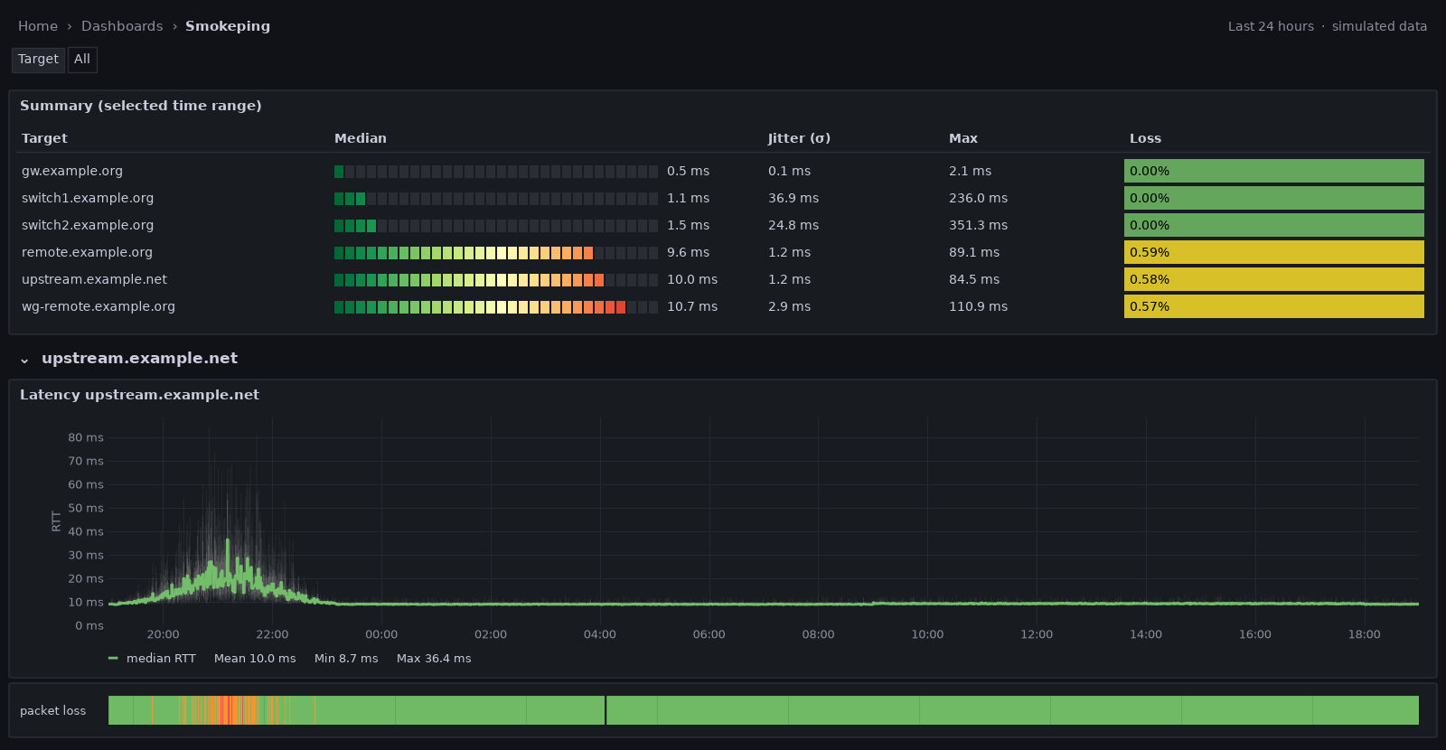
With the variable set to refresh on time range change, new targets appear as soon as they have data, and removed ones disappear once they’re out of the visible range. A summary table at the top shows every target with its median, jitter (σ), worst round trip and packet loss for the selected range.

What the first data shows

Even the first quarter of an hour, with every target at 0 % loss, showed things an average wouldn’t.

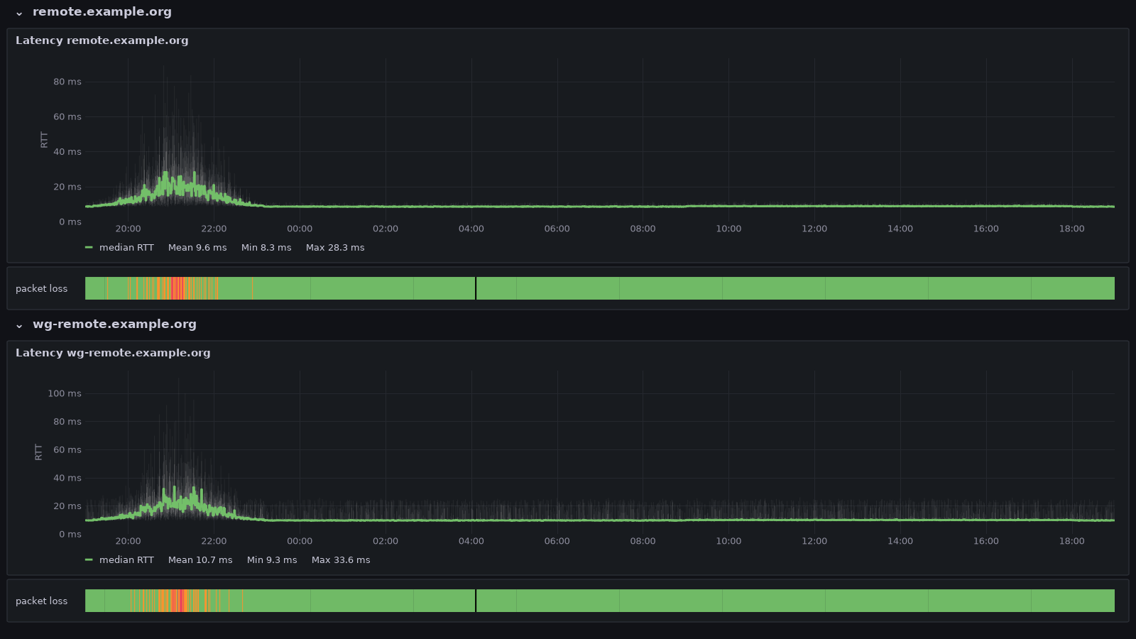
The WireGuard tunnel costs about a millisecond, and some stability. remote and wg-remote are the same server, once reached directly and once through a WireGuard tunnel. The median rises from 8.5 to 9.6 ms, and the jitter roughly triples, from 0.4 to 1.2 ms, with single pings reaching 25 ms. In the graph the direct path is a tight band, while the tunnel’s smoke regularly shoots up.

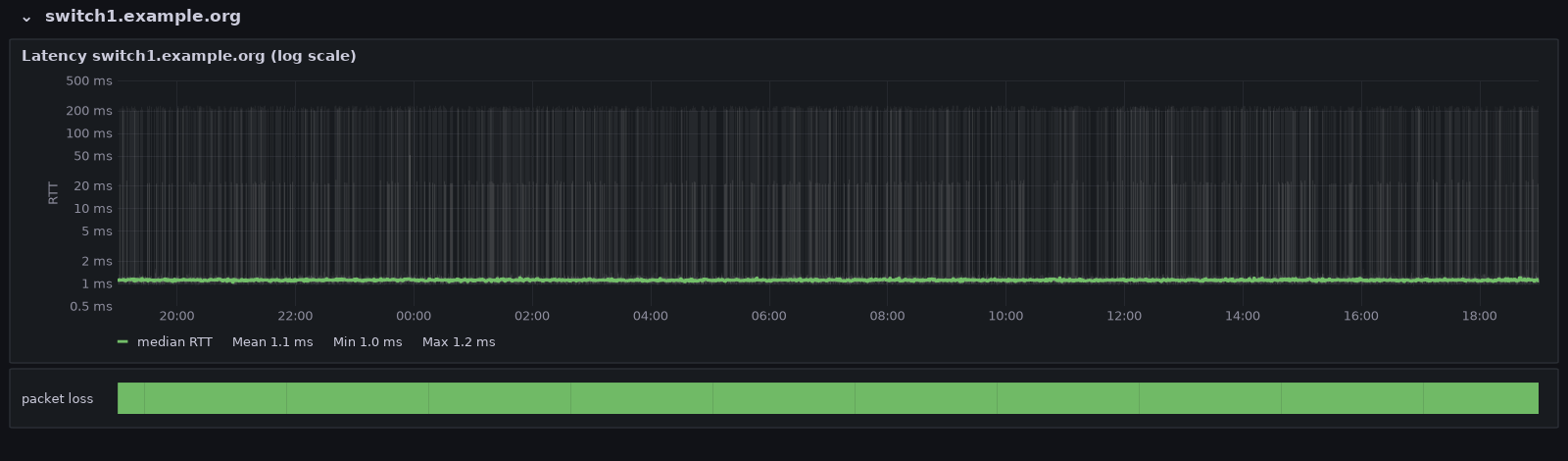
Two 24-hour smoke graphs with simulated data: remote.example.org reached directly, a flat median around 8.5 ms, and wg-remote.example.org through WireGuard, about 1 ms higher with grey smoke spikes to around 20 ms all day. Both rise together during the evening congestion around 21:00 and both show the 04:05 reconnect in their loss strips. — Simulated 24 hours based on the measured baselines: the same server directly (top) and through WireGuard (bottom). The tunnel adds about 1 ms and constant extra smoke; the evening congestion hits both.

Switches answer pings with their slowest component. Both managed switches have a median of about 1 ms, but in many bursts the slowest reply takes 100 to 350 ms. Ping on a switch is answered by its small management CPU, not by the switching hardware, and that CPU has better things to do. Traffic through the switch isn’t affected. On a linear axis those outliers squash everything else into a flat line at the bottom; a logarithmic Y axis (Axis → Scale → Logarithmic) shows the median, the tight core and the outliers at once.

24-hour smoke graph of switch1.example.org on a logarithmic axis with simulated data: the median stays at about 1 ms the whole day, thin grey smoke lines from single slow replies reach about 200 ms throughout, and the packet-loss strip is green from start to end. — Simulated 24 hours based on the measured baseline: a managed switch on a logarithmic axis. The ~1 ms median never moves, the management CPU’s slow replies appear all day, and the evening congestion upstream doesn’t touch it.

The firewall answers in a median of 0.5 ms, and the upstream reference host in a steady 8.9 ms with about 0.4 ms of jitter. That’s the baseline I want to have when the next “the internet is slow” complaint comes in.

What a bad evening looks like

A quarter of an hour of calm data doesn’t show what the graph is for. The probe hasn’t been running long enough to catch a real incident yet, so the 24-hour screenshots in this post use simulated data: generated from the baselines measured above (median, spread and outliers per host), with two typical incidents added on the internet path only.

Evening congestion. From about 19:40 the median to the upstream host creeps up, peaks around 21:00 at three to four times its normal value, and is back to normal by 23:00. Before the median moves much, the smoke gets taller: the pings within each burst scatter more, the first sign of filling queues. At the peak the loss strip turns yellow, orange and briefly red.
The nightly reconnect. At 04:05 the line is down for two minutes, a forced PPPoE reconnect that some providers still do once a day. In the loss strip it shows as a thin black mark.

The useful part is the comparison across targets. The gateway and both switches stay flat through the whole evening, while every target behind the uplink rises at the same time. That puts the problem upstream, at the provider, not in the LAN, the firewall or the remote server. An average wouldn’t have shown it: over the full 24 hours the upstream median comes out at 10.0 ms, barely above its 8.9 ms baseline. I’ll replace the simulated screenshots with real ones once the probe has caught a real bad evening.

SmokePing vs. this setup

	SmokePing	Telegraf + InfluxDB + Grafana
Probe	fping and many other probes (DNS, HTTP, …)	Telegraf `inputs.ping`; other Telegraf inputs for DNS or HTTP
Distribution	all 20 values stored	min, p10, p25, p50, p75, p90, max
Loss	colours the median line	separate state timeline below the graph
Storage	RRD, fixed consolidation	InfluxDB with your own retention
Extra software	SmokePing, web server, CGI	none, if the stack already runs
Alerting	built-in patterns	Grafana alerting on the same data

SmokePing still has more probe types and keeps every single value. But if Telegraf, InfluxDB and Grafana are already running, a dozen lines of Telegraf config and one dashboard give 90 % of the picture, on the same screen as everything else, and ready for Grafana alerting.